Software Architecture¶

Task Diagram¶

The robot runs nine concurrent tasks under a cooperative round-robin scheduler (cotask). Tasks communicate exclusively through shared variables and queues (task_share), with no direct function calls between tasks.

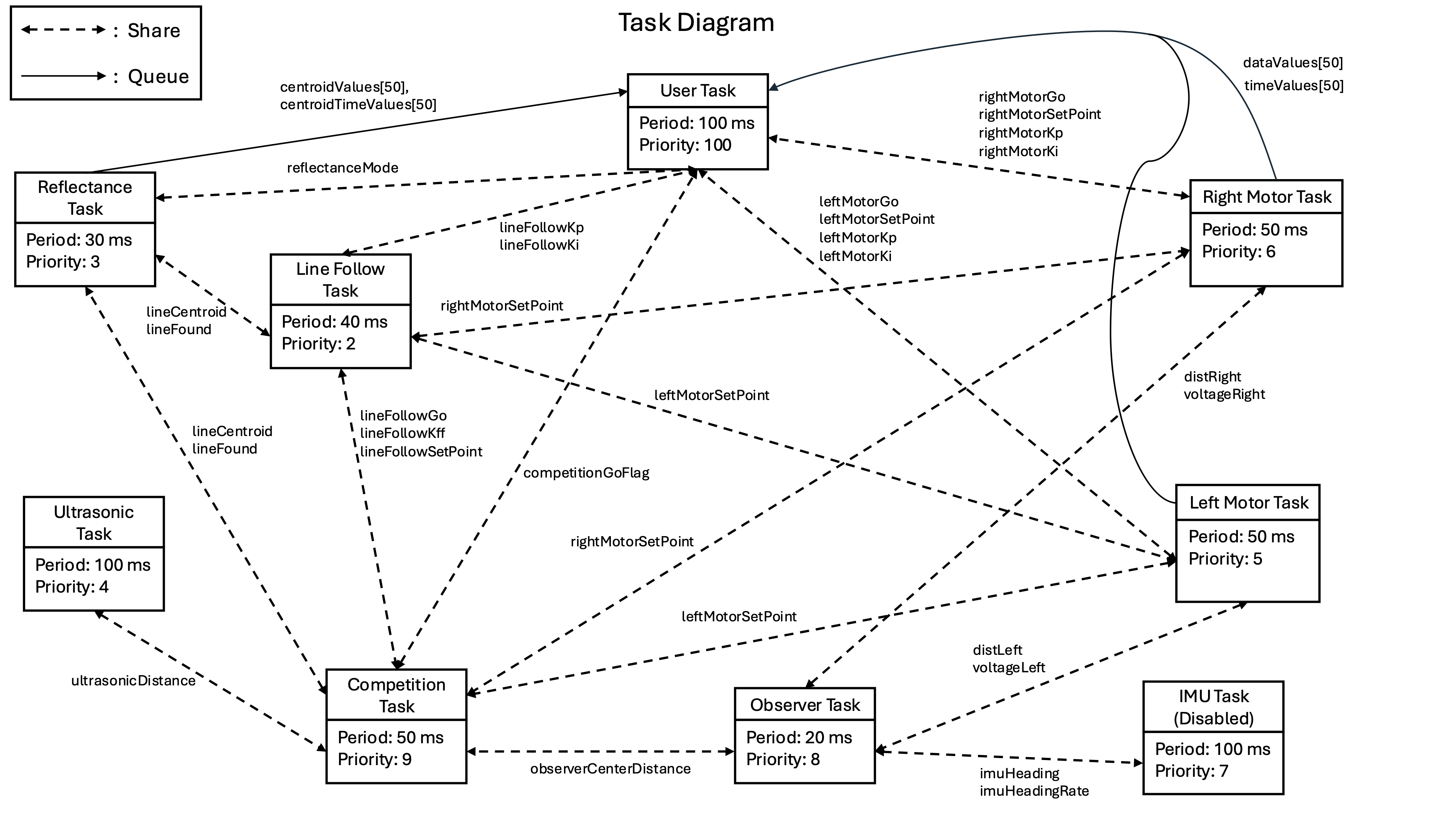
Task Summary¶

Task	Period	Priority	Role
`task_user`	100 ms	100	Serial UI, command dispatch
`task_motor` (left)	50 ms	5	PI velocity control, left wheel
`task_motor` (right)	50 ms	6	PI velocity control, right wheel
`task_reflectance`	30 ms	3	Line sensor calibration & centroid
`task_line_follow`	40 ms	2	Steering PI + feed-forward
`task_imu`	100 ms	7	Heading & heading-rate (disabled at competition)
`task_ultrasonic`	100 ms	4	Distance measurement
`task_observer`	20 ms	8	Center distance estimate
`task_competition`	50 ms	9	Course sequencer (15-state FSM)

Control Scheme¶

Motor Velocity Control¶

The discrete-time PI controller (implemented in controller.py) computes:

\[u(k) = K_p \, e(k) + K_i \sum_{j=0}^{k} e(j) \, \Delta t\]

with conditional anti-windup: the integrator is held constant whenever the output is saturated and further integration would deepen the saturation. Output is clamped to ±100% duty cycle.

Tuned gains:

Parameter	Value
\(K_p\)	0.15
\(K_i\)	4.0
Saturation	±100 % duty cycle

Line-Following Controller¶

The line-following controller steers the robot by applying a differential speed correction proportional to the centroid error:

\[\text{left speed} = v_{nominal} + u_{LF}\]

\[\text{right speed} = v_{nominal} - u_{LF}\]

where \(u_{LF}\) is the PI controller output driven by the reflectance centroid (range −1 to +1, where 0 = centered on line). The actuator gain scales the correction to mm/s using the effective wheel-to-wheel width of 141 mm.

A feed-forward term assists with curved track segments:

\[u_{FF} = K_{ff} \cdot \omega_{ff}, \quad \omega_{ff} = \frac{v_{nominal}}{r_{curve}}\]

Tuned gains:

Parameter	Value	Notes
\(K_p\)	0.40	Steering proportional gain
\(K_i\)	0.30	Integral anti-drift
\(K_{ff}\) (straight)	0.0	No feed-forward on straights
\(K_{ff}\) (tight curve, R125)	0.6	Aggressive assist
\(K_{ff}\) (gentle curve)	0.3	Moderate assist
Saturation	±100 mm/s correction

State Observer¶

A discrete-time Luenberger observer was designed offline for the robot’s linearized model. The state vector is:

\[\begin{split}\hat{x} = \begin{bmatrix} d_{center} \\ \psi \\ \omega_L \\ \omega_R \end{bmatrix}\end{split}\]

with the update equations:

\[\hat{x}_{k+1} = A_D \hat{x}_k + B_D u_k, \qquad \hat{y}_k = C_D \hat{x}_k\]

\[\begin{split}A_D = \begin{bmatrix} 0.3799 & 0 & 0.3486 & 0.3486 \\ 0 & 0.0000029 & 0 & 0 \\ -0.1694 & 0 & 0.1103 & 0.1103 \\ -0.1694 & 0 & 0.1103 & 0.1103 \end{bmatrix}\end{split}\]

\[\begin{split}B_D = \begin{bmatrix} 0.866 & 0.866 & 0.310 & 0.310 & 0 & 0 \\ 0 & 0 & -0.007 & 0.007 & 0.0001 & 0.004 \\ 1.143 & 0.842 & 0.085 & 0.085 & 0 & -1.827 \\ 0.842 & 1.143 & 0.085 & 0.085 & 0 & 1.827 \end{bmatrix}\end{split}\]

\[\begin{split}C_D = \begin{bmatrix} 1 & -70 & 0 & 0 \\ 1 & 70 & 0 & 0 \\ 0 & 1 & 0 & 0 \\ 0 & 0 & -0.25 & 0.25 \end{bmatrix}\end{split}\]

The observer task runs at 20 ms to match the model’s discretization period. In competition, the full observer was replaced with a simple wheel-average estimator for reliability:

\[d_{center} = \frac{d_L + d_R}{2}\]

Algorithms & Design Decisions¶

Cooperative Multitasking¶

Each task is a Python generator function that calls yield at least once per iteration, returning control to the cotask scheduler. The scheduler runs each task at its configured period using priority-based round-robin scheduling. Inter-task data is exchanged through 41 Share objects (single-value, interrupt-safe) and 4 50-element Queue buffers for time-series logging. Configuration (PI gains, IMU calibration offsets) is persisted to gains.json and imu.json on the MCU filesystem so settings survive power cycles.

Reflectance Centroid Calculation¶

Each of the 7 IR sensors is first normalized using a two-point calibration:

\[v_i = \text{clamp}\!\left(\frac{r_i - r_{dark,i}}{r_{light,i} - r_{dark,i}},\ 0,\ 1\right)\]

where \(r_i\) is the averaged raw ADC reading (averaged over 5 reads per cycle to reduce noise), and \(r_{dark,i}\), \(r_{light,i}\) are per-sensor dark and light reference values captured during calibration. The result is 0 for a white surface and 1 for the black line.

The line position is then computed as a weighted centroid:

\[C = \frac{\sum_{i=1}^{7} w_i \cdot v_i}{\sum_{i=1}^{7} v_i}, \qquad w = [-3,\ -2,\ -1,\ 0,\ 1,\ 2,\ 3]\]

\(C\) ranges from −3 (line at far left) to +3 (line at far right), with 0 meaning centered. For the line-following controller the output is divided by 3 to normalize to [−1, +1].

Line-loss detection uses the sum of calibrated values \(S = \sum v_i\). If \(S < 1.0\) (all sensors read white — line not found) or \(S > 6.85\) (all sensors read black — sensor off track), the line is considered lost and the last valid centroid is returned instead.

Calibration the robot is placed on a light surface, then a dark surface, and each phase collects 100 samples at 10 ms intervals. Per-sensor averages are stored to ir_calibration.json on the MCU filesystem and reloaded on startup.